This document will give a detailed introduction into the writing of DRC runsets. See also DRC Reference for a full reference of the DRC functions.
Runsets are basically Ruby scripts running in the context of a DRC runset interpreter. On that level, DRC runsets work with very few classes, specifically:
Some functions are provided on global level and can be used without any object.
The basic elements of runsets are input and output specifications. Input is specified through "input" method calls. "input" will create a layer object that contains the shapes of specified layer. The results are output by calling the "output" method on a layer object with a specification where the output shall be sent to.
In general, the runset language is rich in alternatives - often there are more than one way to achieve the same result.
The script is executed in immediate mode. That is, each function will immediately be executed and the results of the operations can be used in conditional expressions and loops. Specifically it is possible to query whether a layer is empty and abort a loop or skip some block in that case.
Being Ruby scripts running in KLayout's scripting engine environment, runsets can make use of KLayout's full database access layer. It is possible to manipulate geometrical data on a per-shape basis. For that purpose, methods are provided to interface between the database access layer ("RBA::..." objects) and the DRC objects ("DRC::..." objects). Typically however it is faster and easier to work with the DRC objects and methods.
The DRC script language is based on Ruby which delivers many native language features. Basically, inside a script you can include another script through "load". This will read a file and execute the content of this file in the context of the script it is loaded into.
Unfortunately, "load" creates a local context for variables. Hence it's not possible for example to use "load" to read a file that defines variables for further use in the DRC script.
To overcome this problem, KLayout offers a specific extension which embeds another file into the source by employing some kind of preprocessing. This way, a file can be included into another one like it was pasted at this place.
The notation is this:
# %include to_include.drc
which will include "include.drc". If no absolute path is given, this file is looked up relative to the file it is included in.
The file name can be put in quotes as well. Expression interpolation is supported (for the notation see About Expressions). Hence it is possible to access environment variables for example like this:
# %include $(env("HOME"))/to_include.drc
Because Ruby does not see the original files, some internals (e.g. introspection) will report wrong file names and line numbers. In most cases - for example when using "__FILE__" or "__LINE__" or when receiving stack traces and errors - the file names and line numbers will correctly refer to the source files before include file processing.
Input is specified with the "input" method or global function. "input" is basically a method of a source object. There is always one source object which is the first layout loaded into the current view. Using "input" without and source object is calling that method on that default source object. As source is basically a collection of multiple layers and "input" will select one of them.
"input" will create a layer object representing the shapes of the specified input layer. There are multiple ways to specify the layer from which the input is taken. One of them is by GDS layer and datatype specification:
# GDS layer 17, datatype 0
l = input(17)

# GDS layer 17, datatype 10
l = input(17, 10)

# By expression (here: GDS layers 1-10, datatype 0 plus layer 21, datatype 10)
# All shapes are combined into one layer
l = input("1-10/0", "21/10")
Input can be obtained from other layouts than the default one. To do so, create a source object using the "layout" global function:
# layer 17 from second layout loaded
l = layout("@2").input(17)

# layer 100, datatype 1 and 2 from "other_layout.gds"
other_layout = layout("other_layout.gds")
l1 = other_layout.input(100, 1)
l2 = other_layout.input(100, 2)
Output is by default sent to the default layout - the first one loaded into the current view. The output specification includes the layer and datatype or the layer name:
# send output to the default layout: layer 17, datatype 0
l.output(17, 0)

# send output to the default layout: layer named "OUT"
l.output("OUT")

# send output to the default layout: layer 17, datatype 0, named "OUT"
l.output(17, 0, "OUT")
Output can be sent to other layouts using the target function:
# send output to the second layout loaded:
target("@2")

# send output to "out.gds", cell "OUT_TOP"
target("out.gds", "OUT_TOP")
Output can also be sent to a report database using the report function:
# send output to a report database with description "Output database"
# - after the runset has finished this database will be shown
report("Output database")

# send output to a report database saved to "drc.lyrdb"
report("Output database", "drc.lyrdb")
When output is sent to a report database, the specification must include a formal name and optionally a description. The output method will create a new category inside the report database and use the name and description for that:
# specify report database for output
report("The output database")
...
# Send data from layer l to new category "check1"
l.output("check1", "The first check")
The report and target specification must appear before the actual output statements. Multiple report and target specifications can be present sending output to various layouts or report databases. Note that each report or target specification will close the previous one. Using the same file name for subsequent reports will not append data to the file but rather overwrite the previous file.
Layers that have been created using "output" can be used for input again, but care should be taken to place the input statement after the output statement. Otherwise the results will be unpredictable.
It is possible to open "side" reports and targets and send layers to these outputs without closing the default output.
To open a "side report", use new_report in the same way you use "report". Instead of switching the output, this function will return a new report object that can be included in the argument list of "output" for the layer that is to be sent to that side report:
# opens a new side report
side_report = new_report("Another report")
...
# Send data from layer l to new category "check1" to the side report
l.output(side_report, "check1", "The first check")
In the same way, "side targets" can be opened using new_target. Such side targets open a way to write certain layers to other layout files. This is very handy for debugging:
# opens a new side target for debugging
debug_out = new_target("debug.gds")
...
# Send data from layer l to the debug output, layer 100/0
l.output(debug_out, 100, 0)
Dimension specifications are used in many places: for coordinates, for spacing and width values and as length values. In all places, the following rules apply:
Units are added using the unit methods:
Area units are usually square micrometers. You can use units as well to indicate an area value in some specific measurement units:
Angles are always given in degree units. You can make clear that you want to use degree by adding the degree unit method:
Runsets are basically scripts written in an object-oriented language. It is possible to write runsets that don't make much use of that fact, but having a notion of the underlying concepts will result in better understanding of the features and how to make full use of the capabilities.
In KLayout's DRC language, a layer is an object that provides a couple of methods. The boolean operations are methods, the DRC functions are methods and so on. Method are called "on" an object using the notation "object.method(arguments)". Many methods produce new layer objects and other methods can be called on those. The following code creates a sized version of the input layer and outputs it. Two method calls are involved: one sized call on the input layer returning a new layer object and one output call on that object.
input(1, 0).sized(0.1).output(100, 0)
The size method like other methods is available in two flavors: an in-place method and an out-of-place method. "sized" is out-of-place, meaning that the method will return a new object with the new content but not modify the object. The in-place version is "size" which modifies the object. Only the layer object is modified, not the original layer.
The following is the above code written with the in-place version:
layer = input(1, 0)
layer.size(0.1)
layout.output(100, 0)
Using the in-place versions is slightly more efficient in terms of memory since with the out-of-place version, KLayout will keep the unmodified copy as long as there is a chance it may be required. On the other hand the in-place version may cause strange side effects since because of the definition of the copy operation: a simple copy will just copy a reference to a layer object, not the object itself:
layer = input(1, 0)
layer2 = layer
layer.size(0.0)
layer.output(100, 0)
layer2.output(101, 0)
This code will produce the same sized output for layer 100 and 101, because the copy operation "layer2 = layer" will not copy the content but just a reference: after sizing "layer", "layer2" will also point to that sized layer.
That problem can be solved by either using the out-of-place version or by creating a deep copy with the "dup" function:
# out-of-place size:
layer = input(1, 0)
layer2 = layer
layer = layer.sized(0.0)
layer.output(100, 0)
layer2.output(101, 0)

# deep copy before size:
layer = input(1, 0)
layer2 = layer.dup
layer.size(0.0)
layer.output(100, 0)
layer2.output(101, 0)
Some methods are provided in different flavors including function-style calls. For example the width check can be written in two ways:
# method style:
layer.width(0.2).output("width violations")

# function style:
w = width(layer, 0.2)
output(w, "width violations")
The function style is intended for users not familiar with the object-oriented style who prefer a function notation.
Here is a brief overview over some of the methods available:
KLayout knows four layer types: polygon, edge, edge pair and text layers. Polygon and edge layers are the basic layer types for geometrical operations.
Polygon layers are created from original layers using input or polygons. "input" will also turn texts into small polygons with a size of 2x2 DBU while "polygons" will skip texts. For handling texts, the labels method is recommended which renders a true text layer. Text layers are described below.
Polygon layers describe objects having an area ("filled objects" in the drawing view). Such objects can be processed with boolean operations, sized, decomposed into holes and hull, filtered by area and perimeter and so on. DRC methods such as width and spacing checks can be applied to polygons in a different way than between different polygons (see space, separation and notch for example).
Polygons can be raw or merged. Merged polygons consist of a hull contour and zero to many hole contours inside the hull. Merging can be ensured by putting a layer into "clean" mode (see clean, clean mode is the default). Raw polygons usually don't have such a representation and consist of a single contour folding inside to form the holes. Raw polygons are formed in "raw" mode (see raw).
Egde layers can be derived from polygon layers and allow the description is individual edges ("sides") of a polygon. Edge layers offer DRC functions similar for polygons but in a slightly different fashion - edges are checked individually, non considering the polygons they belong to. Neither do other parts of the polygons shield interactions, hence the results may be different.
Edges can be filtered by length and angle. extended allows erecting polygons (typically rectangles) on the edges. Edge layers are useful to perform operations on specific parts of polygons, for example width or space checks confined to certain edge lengths.
Edges do not differentiate whether they originate from holes or hulls of the polygon. The direction of edges is always following a certain convention: when looking from the start to the end point of an edge, the "inside" of the polygons from which the edges were derived, is to the right. In other words: the edges run along the hull in clockwise direction and counterclockwise along the holes.
Merged edges are joined, i.e. collinear edges are merged into single edges and degenerate edges (single-point edges are removed). Merged edges are present in "clean" mode (see clean, clean mode is the default).
Polygons can be decomposed into edges with the edges method. Another way to generate edges is to take edges from edge pair objects which are generated by the DRC check functions.
Starting with version 0.27, KLayout offers support for text layers. "Texts" are basically locations with a label, i.e. a dot with an arbitrary string attached. "Text collections" are collections of such objects.
Texts can be used to select polygons or as net names in net extractions.
Text collections are kept in "text layers". These are created using the labels methods instead of "input".
These operations are supported for text layers:
Edge pairs are objects consisting of two edges. Edge pairs are handy when discribing a DRC check violation, because a violation occurs between two edges. The edge pair generated for such a violation consists of the parts of both edges violation the condition. For two-layer checks, the edges originate from the original layers - edge 1 is related to input 1 and edge 2 is related to input 2.
Edge pair collections act like normal layers, but very few methods are defined for those. Edge pairs can be decomposed into single edges (see edges, first_edges and second_edges).
Edge pairs can be converted to polygons using polygons. Edge pairs can have a vanishing area, for example if both edges are coincident. In order to handle such edge pairs properly, an enlargement can be applied optionally. With such an enlargement, the polygon will cover a region bigger than the original edge pair by the given enlargement.
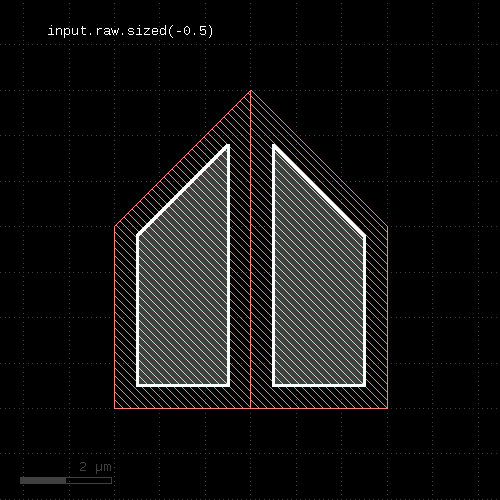
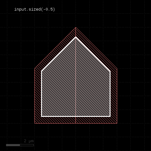
KLayout's DRC engine supports two basic ways to interpret geometrical information on a layer: in clean mode, polygons or edges are joined if they touch. If regions are drawn in separate pieces they are effectively joined before they are used. In raw mode, every polygon or shape on the input layer is considered a separate part. There are applications for both ways of looking at a set of input shapes, and KLayout supports both ways.
Clean mode is the default - every layer generated or taken from input will be used in clean mode. To switch to raw mode, use the "raw" method. "raw mode" is basically a flag set on the layer object which instructs the engine not the merge polygons prior to use. The raw mode flag can be reset with the "clean" method.
Most functions implicitly merge polygons and edges in clean mode. In the documentation this fact is referred to as "merged semantics": if merged semantics applies for the function, coherent polygons or edges are considered one object in clean mode. In raw mode, every polygon or edge is treated as an individual object.
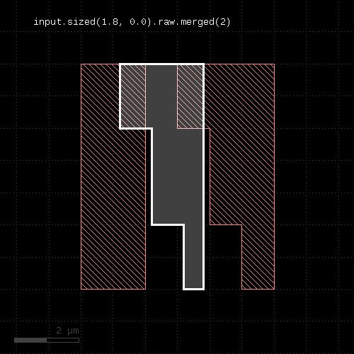
One application is the detection of overlapping areas after a size step:
overlaps = layer.size(0.2).raw.merged(2)
That statement has the following effect:

The "merged" method with an argument of 2 will produce output where more than two polygons overlap. The size function by default creates a clean layer, but separate polygons for each input polygon, so by using "raw", the layer is switched into raw mode that makes the individual polygons accessible without merging them into one bigger polygon.
Please note that the raw or clean methods modify the state of a layer so beware of the following pitfall:
layer = input(1, 0)
layer.raw.sized(0.1).output(100, 0)

# this check will now be done on a raw layer, since the
# previous raw call was putting the layer into raw mode
layer.width(0.2).ouput(101, 0)
The following two images show the effect of raw and clean mode:
 |  |
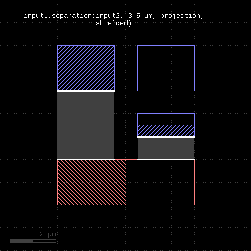
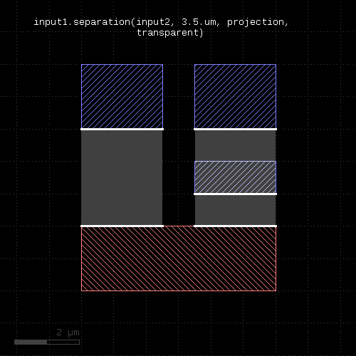
"Shielding" is a concept where DRC measurements do not "look through" layout features. With shielding, a DRC violation is skipped when another feature would (fully) block the violation marker's path. Shielding is available and enabled by default for the (internal or external) distance-based DRC functions: width, space, separation (sep), notch, isolated (iso), enclosing (enc) or enclosed or overlap. Shielding is turned off using the "transparent" option or turned on using "shielded". The latter is only for clarity, but is not required as shielding is enabled by default.
The following examples demonstrate the effect of shielding: in the right example, shielding is turned off. Hence, the violation between the upper box on the right and the lower bar is no longer shielded by the small bar between them and this additional violation is reported too.
 |  |
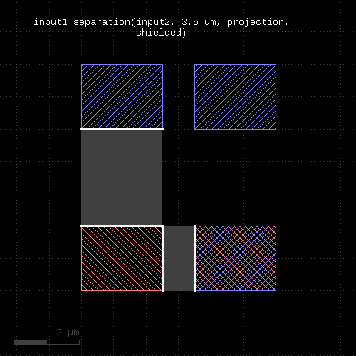
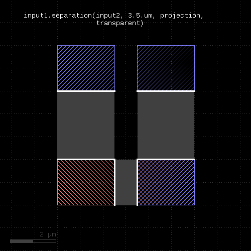
Although shielding feels more natural, it can have an adverse effect as it is effective at zero distance already. In the following example, the second layer is a subset of the first. When testing the distance between second and first, the overlapping first layer shapes will block the separation measurement in shielded mode. Hence, only transparent mode will render the actual distance violation. The bottom right blue box is not shielded by the overlaying red box:
 |  |
Starting with version 0.27, the DRC language got a new feature which is "universal DRC".
On one hand, this is a more convenient way to write DRC checks because it allows specifications using natural compare operators. For example, the following plain width check
...
drc_w = input(1, 0).width(0.2)
...
can be written as:
...
drc_w = input(1, 0).drc(width < 0.2)
...
The drc method is the "universal DRC" method. It takes an operator. In the simple case, this operator is a simple constraint of the form "measurement < value", but it supports a number of different variants:
"measurement" is "width", "notch", "isolated" ("iso"), "separation" ("sep"), "overlap", "enclosed" or "enclosuring" ("enc"). The last three checks are two-layer checks which require a second layer. The second layer is specified together with the measurement like this:
...
l1 = input(1, 0)
l2 = input(2, 0)
drc_sep = l1.drc(separation(l2) <= 0.5)
...
Options are also specified together with the measurement and follow the same notation as the plain methods. For example to specify "projection" metrics, use:
...
drc_w = input(1, 0).drc(width(projection) < 0.2)
...
However, the universal DRC is much more than a convenient way to write checks: it offers a number of options to further process the results. The functionality behind the universal DRC function is basically a kind of loop over all primary shapes (the ones from the layer the "drc" function is called on). The operations in the drc function's brackets is executed on each of the primary shapes where the neighborhood of that single shape is considered. This scheme is more efficient and enables applications beyond the capabilities of the plain layer methods.
For example, the boolean "&" operator implements a "local" boolean AND inside this loop. This allows to efficiently check for both space and width violations:
...
drc_ws = input(1, 0).drc((width < 0.2) & (space < 0.3))
...
The boolean AND is computed between the edges on the primary shape and returns the parts where both space and width violations are flagged. The boolean operation is more efficient than the plain alternative:
...
drc_ws1 = input(1, 0).width(0.2).edges
drc_ws2 = input(1, 0).space(0.3).edges
drc_ws = drc_ws1 & drc_ws2
...
The reason is that performing the boolean computation in the local loop can be shortcut if one inputs is empty. It does not need to store a (potentially big) edge set with edges as produced by the plain-method implementation. Instead it will work with a temporary and local edge set only and free the memory space as soon as it moves on to the next primary shape.
Overall, the universal DRC function is a rich feature and offers filters based on polygons or edge properties, polygon or edge manipulation operators, conditionals and a lot more. For more details see the drc function documentation.
While the runset is executed, a log is written that lists the methods and their execution times. The log is enabled using the verbose function. The log and info functions allows entering additional information into the log. "info" will enter the message if verbose mode is enabled. "log" will enter the message always. silent is equivalent to "verbose(false)".
The log is shown in the log window or - if the log window is not open - on the terminal on Linux-like systems.
The log function is useful to print result counts during processing of the runset:
...
drc_w = input(1, 0).width(0.2)
log("Number of width violations: #{drc_w.data.size}")
...
The error function can be used to output error messages unconditionally, formatted as an error. The log can be sent to a file instead of the log window or terminal output, using the log_file function:
log_file("drc_log.txt")
verbose(true)
info("This message will be sent to the log file")
...
The profile function will collect profiling information during the DRC run. At the end of the script, the operations are printed to the log output, sorted by their CPU time and approximate memory footprint. "profile" can be given a numerical argument indicating the number of operations to print. Lower-ranking operations are skipped in that case. By default, all operations are printed.
# enables profiling
profile
...
Tiling is a method to reduce the memory requirements for an operation. For big layouts, pulling a whole layer into the engine is not a good idea - huge layouts will require a lot of memory. The tiling method cuts the layout into tiles with a given width and height and processes them individually. The tiling implementation of KLayout can make use of multiple CPU cores by distributing the jobs on different cores.
Tiling does not come for free: some operations have a potentially infinite range. For example, selecting edges by their length in clean mode basically requires to collect all pieces of the edge before the full length can be computed. An edge running over a long length however may cross multiple tiles, so that the pieces within one tile don't sum up to the correct length.
Fortunately, many operations don't have an infinite range, so that tiling can be applied successfully. These are the boolean operations, sizing and DRC functions. For those operations, a border is added to the tile which extends the region inside which the shapes are collected. That way, all shapes potentially participating in an operation are collected. After performing the operation, polygons and edges extending beyond the tile's original boundary are clipped. Edge pairs are retained if they touch or overlap the original tile's border. That preserves the outline of the edge pairs, but may render redundant markers in the tile's border region.
For non-local operations such as the edge length example, a finite range can be deduced in some cases. For example, if small edges are supposed to be selected, the range of the operation is limited: longer edges don't contribute to the output, so it does not matter whether to take into account potential extensions of the edge in neighboring tiles. Hence, the range is limited and a tile border can be given.
To enable tiling use the tiles function. The threads function specifies the number of CPU cores to use in tiling mode. flat will disable tiling mode:
# Use a tile size of 1mm
tiles(1.mm)
# Use 4 CPU cores
threads(4)

... tiled operations ...

# Disable tiling
flat

... non-tiled operations ...
Some operations implicitly specify a tile border. If the tile border is known (see length example above), explicit borders can be set with the tile_borders function. no_borders will reset the borders (the implicit borders will still be in place):
# Use a tile border of 10 micron:
tile_borders(10.um)

... tile operations with a 10 micron border ...

# Disable the border
no_borders
A word about the tile size: typically tile dimensions in the order of millimeters is sufficient. Leading-edge technologies may require smaller tiles. The tile border should not be bigger than a few percent of the tile's dimension to reduce the redundant tile overlap region. In general using tiles is a compromise between safe function and performance. Very small tiles imply some performance overhead do to shape collection and potentially clipping. In addition, the clipping at the tile's borders may introduce artificial polygon nodes and related snapping to the database unit grid. That may not be desired in some applications requiring a high structure fidelity. Hence, small tiles should be avoided in that sense too.
Alternatively to the tiling option, hierarchical mode is available. In hierarchical mode, the DRC functions operate on subcells if their configuration allows this. The algorithm will automatically detect whether an operation can be performed in a subcell. For example, a sizing operation can be done inside a subcell, if the cell's content is not connected to anything outside the cell.
To enable hierarchical operations, use the "deep" statement:
report("deep 2")

# enable deep (hierarchical) operations
deep

poly = input(3)

spc = poly.space(0.5)
spc.output("poly space >0.5")
"deep" is not compatible with tiling. "tiles" will disable "deep" and vice versa. To disable deep mode, use "flat".
Deep processing is a layer property. After "deep" has been specified, layers derived with "input" are declared to be deep - i.e. hierarchical operations are enabled on them. Operations on deep layers will usually render other deep layers. This is also true for edge and edge pair layers. For example, the "space" operation above will render a hierarchical edge pair layer.
In binary operations such as boolean operations, the operation is performed hierarchically, if both involved layers are deep. A layer can be explicitly converted to a flat layer using "flatten".
To check whether a layer is deep, use "is_deep?".
report("deep 2")

# enable deep (hierarchical) operations
deep

poly = input(3)
puts poly.is_deep?   # -> true
poly.flatten
puts poly.is_deep?   # -> false
Most operations are hierarchy enabled, with a few exceptions. Some operations - specifically the transformation operations such as "move", "rotate" and the anisotropic sizing or the grid snap operations will generate cell variants. Such variants reflect different configurations of cells with respect to the requested operation. For example, with anisotropy (x != y), rotated cells need to be treated differently from non-rotated ones. In the "snap" feature, cell variants are created if the cell's instances are not all on-grid. Most functions need to create variants only when the same cell is instantiated with different magnification factors.
When writing back a layout with cell variants, new versions of cells will appear.
When sending the output of hierarchical operations to a report database, the markers will be listed under the cell name they appear. A sample cell instance is provided within the marker database to allow visualizing the marker in at least one context.
Functions which require merged polygons utilize the net clustering algorithm to form the merged polygons. All connected shapes are collected and merged into a bigger polygon. This happens in the lowest possible level on the hierarchy where the shape clusters are complete. In some cases - when the shapes come from big coherent regions - this may happen on the top cell level and the resulting polygon will be very big. This will lead to poor performance.
The DRC's hierarchical mode will - except for cell variants in the cases mentioned - not modify the cell hierarchy. This hierarchy-preserving nature is good for certain applications, but leads to a compromise in terms of resolving hierarchically different configurations. As the algorithm is not allowed to create variants in most cases, the only remaining option is to propagate results from such cases into the parent cells. In the worst case this will lead to flattening of the layout and loss of hierarchy.
The DRC feature has some support for user properties. User properties are sets of key/value pairs attached to shapes. This is a standard feature of KLayout and GDS/OASIS. The GDS format supports numerical (positive integer) keys and string values while OASIS supports more types of keys and values - specifically string keys.
For DRC, the property set attached to a shape is regarded as a whole. The DRC can act on these properties in specific ways:
Specifically, DRC functions can also generate properties. Currently there is only the "nets" method which attaches net identity information to shapes involved in a "connect" statement. This feature opens a path to implementing "connected" or "unconnected" mode boolean operations and DRC checks.
As of this writing, user property support is somewhat experimental. User properties support has a huge potential, so there is more to come.
Currently, the following operations can be conditioned to act on shapes with same or different properties:
A variety of operations can transfer properties, i.e. edge-pair-to-polygon, edge-pair-to-edges, polygon-to-edges, edge-to-polygon, some filters, the "size" function. It is planned to enable most features to transfer properties where applicable.
Property generation is supported currently by:
Property manipulation is supported in a very basic way: properties can be removed entirely from a layer or certain property keys can be selected and optionally mapped to a different key. Property values cannot be manipulated currently.
In general, once a layer has properties, shapes with different properties are regarded as non-interacting. When shapes are merged, only groups of shapes with the same properties are merged into bigger chunks. This applies to polygons and edges. This can have the strange consequence that after merge, still polygons may overlap. Note that this only applies to the case with properties. The normal behavior is not changed.
By default, user properties are not read into the shape containers. You need to enable them explicitly:
l1 = input(1, 0, enable_props)
At this point you can select certain keys from the set of properties. For example to select only values with key 17 and 18 (numerical), use:
l1 = input(1, 0, select_props(17, 18))
You can also select and map keys to other keys, like this:
l1 = input(1, 0, map_props({ 17 => 1, 18 => 18 }))This will map values with key 17 to 1 and read those from 18 while maintaining the key. Values with other keys are ignored. See input function documentation for more details.
Once you have a layer with properties, you can remove them:
layer_without_properties = layer.remove_props
You can also apply select_props or map_props to filter values with certain keys or map keys:
reduced_layer = layer.select_props(17, 18)
reduced_layer = layer.map_props({ 17 => 1, 18 => 18 })The most important application is to use the nets method to generate net identity properties:
connect(metal1, via1)
connect(via1, metal2)

metal1_nets = metal1.nets
By default, a unique net identifier (a tuple of circuit and net name) is generated on property key 0. You can specify the key as well:
metal1_nets = metal1.nets(prop(17))
The "nets" function has a number of options, specifically you can filter certain nets (by name or circuit + name). This makes the "nets" function useful for other purposes too. If you do not need properties then, specify "nil" as the property key:
metal1_vdd_net = metal1.nets(prop(nil), "VDD")
The main purpose of properties is to use them in operations. To confine a boolean operation to shapes with different properties, use the props_ne keyword. To confine a boolean operation to shapes with the same properties, use props_eq:
connect(metal1, via1)
connect(via1, metal2)

metal1_nets = metal1.nets
metal2_nets = metal2.nets

metal1_over_metal2_connected = metal1_nets.and(metal2_nets, props_eq)
metal1_over_metal2_unconnected = metal1_nets.and(metal2_nets, props_ne)
You can also instruct this operation to emit the original properties on the output with props_copy:
result_with_props = metal1_nets.and(metal2_nets, props_eq + props_copy)
Similarly, properties can participate in checks:
connect(metal1, via1)
connect(via1, metal2)

metal1_nets = metal1.nets
metal2_nets = metal2.nets

metal1_space_connected = metal1_nets.space(0.4.um, props_eq)
metal1_space_unconnected = metal1_nets.space(1.um, props_ne)
"props_eq", "props_ne" and "props_copy" are also available on the generic DRC function (drc), which opens new options, e.g. detecting potential short locations ("critical area") between unconnected nets:
connect(metal1, via1)
connect(via1, metal2)

metal1_nets = metal1.nets
metal2_nets = metal2.nets

critical_area = l1_nets.drc(primary.sized(0.2.um) & foreign.sized(0.2.um), props_ne)